Hillshade and hypsometric tint

Terrain is the one part of ezu that needs no vector data at all. A DEM source becomes a ScalarField, and two ops read it: color-ramp for elevation colour, hillshade for shading.

{
  "name": "hillshade",
  "pad": 16,
  "sources": {
    "terrain": {
      "type": "dem",
      "url": "https://terrain.reearth.land/mapterhorn-egm08/terrarium/ellipsoid/{z}/{x}/{y}.webp",
      "encoding": "terrarium",
      "tile-size": 512,
      "max-zoom": 14,
      "neighbor-fetch": true
    }
  },
  "nodes": {
    "dem": { "op": "dem", "source": "terrain" },
    "elevation": {
      "op": "color-ramp", "field": "@dem",
      "stops": [
        { "value": -200, "color": "#9bc8e5" },
        { "value": 0,    "color": "#cce6c8" },
        { "value": 500,  "color": "#e0d8a6" },
        { "value": 1500, "color": "#b89271" },
        { "value": 2500, "color": "#8b6b4a" },
        { "value": 3500, "color": "#f4f1ea" }
      ]
    },
    "shade": { "op": "hillshade", "field": "@dem",
               "azimuth-deg": 315, "altitude-deg": 45,
               "exaggeration": 1.5, "mode": "relief" },
    "out": { "op": "blend", "base": "@elevation", "over": "@shade" }
  },
  "output": "@out"
}

That is the complete hillshade.json. Every asset is remote, so it renders from a URL with no checkout:

ezu tile --style https://raw.githubusercontent.com/reearth/ezu/main/crates/ezu/examples/styles/hillshade.json \
  --tile 11/1813/807 --out fuji.png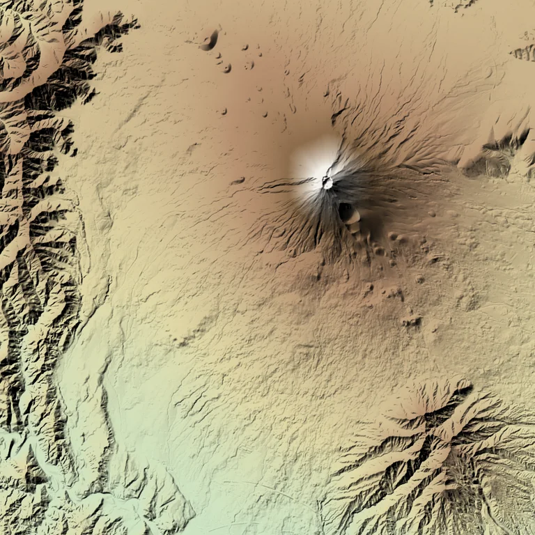

Mount Fuji at z11: a hypsometric ramp under shaded relief, from DEM tiles alone.

The elevation is Re:Earth Terrain’s Mapterhorn-merged global DEM blended with EGM2008 geoid undulations — credit Re:Earth Terrain, Mapterhorn and EGM2008 (NGA) if you render with it. The TileJSON carries that string, so Document::attributions() picks it up without you writing it down.

Get encoding right first

terrarium and mapbox-rgb pack elevation into RGB differently. Point the wrong decoder at a pyramid and you get noise that looks like a rendering bug rather than a configuration one. If your terrain looks like television static, this is why.

Why neighbor-fetch matters

A gradient at the tile’s edge needs elevations from the next tile over. Without the neighbourhood, hillshade steps at every border — a grid of visible seams. The host stitches the 3×3 neighbourhood into one per-tile field before evaluation.

Ask what the source needs rather than assuming: requestedNeighborOffsets('terrain') in wasm, source_neighbor_offsets natively. With neighbor-fetch on — the default — that is all eight, and binding fewer does not simply shrink the neighbourhood: the stitch fills what is missing by clamping the tile’s own edge, so the seam comes back, thinner and harder to spot.

geo_scale is populated on a DEM field, which is what lets hillshade and slope produce real-world angles rather than unitless ones.

Tuning the shading

• azimuth-deg 315 — light from the north-west. This is a cartographic convention, not physics: humans read north-west light as raised and south-east light as sunken. Change it and half your readers will see valleys as ridges.
• altitude-deg — lower is more dramatic and loses detail on flat ground.
• exaggeration — 1.5 is a mild lie that makes gentle terrain legible. Raise it at low zooms where real relief is sub-pixel; drop it towards 1.0 at high zooms where it starts looking inflated.
• mode — relief is the shaded-relief look. Combined with the ramp underneath it gives the classic atlas appearance.

Wire exaggeration to a $param and you can tune it against the map instead of by guesswork.

Ramp stops

Stops are absolute metres, so the same ramp means different things in the Alps and in the Netherlands. Two habits help:

• Put a stop at 0 and one just below it, so the coastline is a hard colour change rather than an interpolated smear.
• Spend your stops where the data is. A ramp with five stops between 0 and 500 m and one at 3500 m reads far better over a coastal region than an evenly spaced one.

Probe the field before you ramp it

The same rule applies to every ScalarField, and it bites hardest on the synthetic ones, whose range is rarely what it looks like. density output is unclamped and scales with intensity. noise values land in [-1, 1], but worley piles up at +1 — over half a tile can be exactly 1.0.

A stop placed outside where a field actually spends its time is simply never reached, and the failure is silent: the ramp appears to do nothing, and turning up opacity does nothing either, because the pixels are already resolving to one end colour.

So look at the distribution first. Point output at a black-to-white ramp over the field, render one tile, and read the histogram back:

"probe": { "op": "color-ramp", "field": "@field",
           "stops": [ { "value": 0, "color": "#000000" },
                      { "value": 1, "color": "#ffffff" } ] }

Pure black means “at or below the low stop”, pure white “at or above the high stop” — so widen the two values until neither is a large share of the tile, and put the real stops where the greys are. Rendering the intermediate node like this is also the fastest way to tell a field that is empty apart from a ramp that is misplaced.

Beyond the classic look

slope yields angle rather than shading, which makes a steepness map:

"steep":  { "op": "slope", "field": "@dem" },
"warn":   { "op": "color-ramp", "field": "@steep",
            "stops": [ { "value": 0, "color": "#00000000" },
                       { "value": 30, "color": "#e0000060" },
                       { "value": 45, "color": "#e00000c0" } ] }

Blend that over a basemap and you have an avalanche-slope overlay. And since a ScalarField is just a field, the painterly ops apply: dither a hypsometric ramp to a small palette for a printed-atlas feel, or run the composite through blur and a paper texture.

A worked example

topo.json reads one DEM three ways at once — contour for vector isolines at a param-driven interval, hillshade for the relief, and slope for cliff shading — over a hypsometric ramp. See it rendered in the gallery.